LaTeX new commands defined for this notebook: $ \newcommand{\bX}{\boldsymbol{X}} \newcommand{\bZ}{\boldsymbol{Z}} \newcommand{\btheta}{\boldsymbol{\theta}} \newcommand{\E}{\mathbb{E}} \newcommand{\L}{\mathcal{L}} \newcommand{\KL}{\operatorname{KL}} \newcommand{\Q}{\mathcal{Q}} $
\bX$\bX$,\bZ$\bZ$,\btheta$\btheta$,\E$\E$,\L$\L$,\KL$\KL$,\Q$\Q$
9.4 The EM Algorithm in General
(Dempster et al., 1977; McLachlan and Krishnan, 1997) EM (expectation maximization) 알고리즘은 잠재변수를 가지는 확률모델에서 모수를 최대우도추정하는 일반적인 방법이다.
확률모델의 관측데이터를 $\bX$, 그리고 잠재변수를 $\bZ$라 할 때, (가우시안 혼합모델에서와 같이) 불완전데이터의 우도함수 $p(\bX|\btheta)$에 비해 완전데이터의 우도함수 $p(\bX,\bZ|\btheta)$를 다루는 것이 비교적 쉽다고 가정하자. 이 경우 주변화(marginalization)로 표현되는 우도함수 $$ p(\bX|\btheta) = \sum_{\bZ} p(\bX,\bZ|\btheta) \tag{9.69} $$ 가 최대가 되는 모수 $\btheta$를 찾고자 하지만, 보통 우도함수가 계산하기 좋은 형태의 식으로 나타나지 않거나 잠재변수 $\bZ$의 구성공간(configuration space)이 너무 방대해서 계산이 어려워진다.
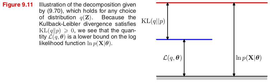
잠재변수 $\bZ$에 대한 임의의 확률분포 $q(\bZ)$에 대해, 하계 $\L(q,\btheta)$와 쿨백-라이블러 발산(Kullback-Leibler divergence) $\KL(q\|p)$을 다음과 같이 정의하면 \begin{align*} \L(q,\btheta) &\equiv \E_\bZ \Bigl[ \ln \Bigl\{ \frac{p(\bX,\bZ|\btheta)}{q(\bZ)} \Bigr\} \Bigr] = \sum_\bZ q(\bZ) \ln \Bigl\{ \frac{p(\bX,\bZ|\btheta)}{q(\bZ)} \Bigr\} \tag{9.71} \\ \KL(q\|p) &\equiv - \E_\bZ \Bigl[ \ln \Bigl\{ \frac{p(\bZ|\bX,\btheta)}{q(\bZ)} \Bigr\} \Bigr] = - \sum_\bZ q(\bZ) \ln \Bigl\{ \frac{p(\bZ|\bX,\btheta)}{q(\bZ)} \Bigr\} \tag{9.72} \end{align*} (9.69)의 로그우도함수는 $$ \ln p(\bX|\btheta) = \L(q,\btheta) + \KL(q\|p) \geq \L(q,\btheta) \tag{9.70} $$
Note: 젠센 부등식(Jensen's inequality)에 따르면 \begin{align*} \KL(q\|p) &= - \E_\bZ \Bigl[ \ln \Bigl\{ \frac{p(\bZ|\bX,\btheta)}{q(\bZ)} \Bigr\} \Bigr] \\ &\geq - \ln \E_\bZ \Bigl[ \frac{p(\bZ|\bX,\btheta)}{q(\bZ)} \Bigr] = - \ln \sum_\bZ q(\bZ) \frac{p(\bZ|\bX,\btheta)}{q(\bZ)} = -\ln \sum_\bZ p(\bZ|\bX,\btheta) = 0 \end{align*}
특히 $q(\bZ)=p(\bZ|\bX,\btheta)$인 경우 $\KL(q\|p)=0$ 이고, 따라서 $\ln p(\bX|\btheta) = \L(q,\btheta)$.
Proof. 베이즈 법칙에 의해 $p(\bZ|\bX,\btheta)p(\bX|\btheta)=p(\bX,\bZ|\btheta)$이고 $\sum_\bZ q(\bZ)=1$이므로 \begin{align*} \ln p(\bX|\btheta) &= \ln \Bigl\{ \frac{p(\bX,\bZ|\btheta)}{p(\bZ|\bX,\btheta)} \Bigr\} = \ln \Bigl\{ \frac{p(\bX,\bZ|\btheta)}{q(\bZ)} \cdot \frac{q(\bZ)}{p(\bZ|\bX,\btheta)} \Bigr\} \\ &= \sum_\bZ q(\bZ) \cdot \left[ \ln \Bigl\{ \frac{p(\bX,\bZ|\btheta)}{q(\bZ)} \Bigr\} - \ln \Bigl\{ \frac{p(\bZ|\bX,\btheta)}{q(\bZ)} \Bigr\} \right] \\ &= \sum_\bZ q(\bZ) \ln \Bigl\{ \frac{p(\bX,\bZ|\btheta)}{q(\bZ)} \Bigr\} - \sum_\bZ q(\bZ) \ln \Bigl\{ \frac{p(\bZ|\bX,\btheta)}{q(\bZ)} \Bigr\} \\ &= \L(q,\btheta) + \KL(q\|p) \end{align*}
결국 로그우도함수 $\ln p(\bX|\btheta)=\L(q,\btheta) + \KL(q\|p)$가 최대가 되는 확률분포 $q(\bZ)$와 모수 $\btheta$를 함께 찾아야 한다. 그런데 임의의 $q(\bZ)$와 $\btheta$에 대해 $\ln p(\bX|\btheta)\geq \L(q,\btheta)$이므로, EM 알고리즘의 일반화는 로그우도함수의 하계 $\L(q,\btheta)$가 최대가 되는 $q(\bZ)$와 $\btheta$를 찾으려 한다.
Review: The General EM Algorithm
Given a joint distribution $p(\bX,\bZ|\btheta)$ over observed variables $\bX$ and latent variables $\bZ$, governed by parameters $\btheta$, the goal is to maximize the likelihood function $p(\bX|\btheta)$ with respect to $\btheta$.
Choose an initial setting for the parameters $\btheta^{old}$.
(E step) Evaluate the posterior distribution of the latent variables given by $p(\bZ|\bX,\btheta^{old})$.
(M step) Evaluate $\btheta^{new}$ given by $$ \btheta^{new} = \arg_\btheta\max\Q(\btheta,\btheta^{old}) \tag{9.32} $$ where the expectation of the complete-data log likelihood evaluated for some parameter $\btheta$ is denoted by $$ \Q(\btheta,\btheta^{old}) \equiv \E_\bZ\bigl[\ln p(\bX,\bZ|\btheta)\bigm| \bX, \btheta^{old} \bigr] = \sum_{\bZ} p(\bZ|\bX,\btheta^{old}) \ln p(\bX,\bZ|\btheta). \tag{9.33} $$
Check for convergence of either the log likelihood or the parameter values. If the convergence criterion is not satisfied, then let $$ \btheta^{old} \leftarrow \btheta^{new} \tag{9.34} $$ and return to Step 2.
(E step) Find $q(\bZ)$ with fixed $\btheta$
(E step)에서는 현재 모숫값 $\btheta^{old}$를 고정한 채 $\L(q,\btheta)$가 최대가 되는 확률분포 $q(\bZ)$를 찾는다.
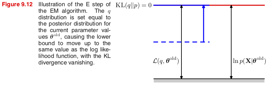
그런데 모숫값 $\btheta^{old}$가 고정되어 있고, $\ln p(\bX|\btheta^{old})$는 $q(\bZ)$에 영향을 받지 않으므로 $\L(q,\btheta^{old})$의 최댓값은 쿨백-라이블러 발산 $\KL(q\|p)=0$이 될 때, 즉 $q(\bZ)=p(\bZ|\bX,\btheta^{old})$일 때이다. (그림 9.12 참조)
(M step) Find $\btheta$ with fixed $q(\bZ)$
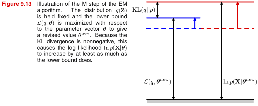
(M step)에서는 앞에서 찾은 확률분포 $q(\bZ)=p(\bZ|\bX,\btheta^{old})$를 고정한 채 $\L(q,\btheta)$가 최대가 되는 새로운 모수 $\btheta^{new}$를 찾는다. \begin{align*} \L(q,\btheta) &\equiv \sum_\bZ q(\bZ) \ln \Bigl\{ \frac{p(\bX,\bZ|\btheta)}{q(\bZ)} \Bigr\} = \sum_\bZ p(\bZ|\bX,\btheta^{old}) \ln \Bigl\{ \frac{p(\bX,\bZ|\btheta)}{p(\bZ|\bX,\btheta^{old})} \Bigr\} \\ &= \sum_\bZ p(\bZ|\bX,\btheta^{old}) \ln p(\bX,\bZ|\btheta) - \sum_\bZ p(\bZ|\bX,\btheta^{old}) \ln p(\bZ|\bX,\btheta^{old}) \\ &= \E_\bZ\bigl[\ln p(\bX,\bZ|\btheta)\bigm| \bX, \btheta^{old} \bigr] - \E_\bZ\bigl[\ln p(\bZ|\bX,\btheta^{old})\bigm| \bX, \btheta^{old} \bigr] \\ &\equiv \Q(\btheta,\btheta^{old}) + \text{const} \tag{9.74} \end{align*}
하계 $\L(q,\btheta^{new})$가 증가함에 따라 로그우도함수 $p(\bX|\btheta^{new})$ 자체도 증가하지만, 모수가 변하기 때문에 ($\btheta^{new}\neq\btheta^{old}$) 더 이상 $\KL(q\|p)=\KL(p(\bZ|\bX,\btheta^{old})\|p(\bZ|\bX,\btheta^{new}))=0$일 보장은 없다. (그림 9.13 참조)
새로운 모수를 구하는 식 (9.33)은 기댓값이므로 총합이 로그 안에 있지 않다는 점에 주목하자. $$ \Q(\btheta,\btheta^{old}) \equiv \E_\bZ\bigl[\ln p(\bX,\bZ|\btheta)\bigm| \bX, \btheta^{old} \bigr] \tag{9.33} $$ 특히 결합확률분포 $p(\bX,\bZ|\btheta)$가 지수족(exponential family)에 속하면 계산에서 로그가 사라지므로 한결 수월하게 모수를 구할 수 있다.
EM always monotonically improves the log-likelihood
Show that $\ln p(\bX|\btheta^{old}) \leq \ln p(\bX|\btheta^{new})$.
Proof. Let $q(\bZ)=p(\bZ|\bX,\btheta^{old})$. From (M step) we have \begin{align*} \L(q,\btheta^{new}) &= \Q(\btheta^{new},\btheta^{old}) - \E_\bZ\bigl[\ln q(\bZ)\bigm| \bX, \btheta^{old} \bigr]\\ &\geq \Q(\btheta^{old},\btheta^{old}) - \E_\bZ\bigl[\ln q(\bZ)\bigm| \bX, \btheta^{old} \bigr] = \L(q,\btheta^{old}) \end{align*} so that $$ \ln p(\bX|\btheta^{new}) \geq \L(q,\btheta^{new}) \geq \L(q,\btheta^{old}) + \KL(q\|q) = \ln p(\bX|\btheta^{old}) $$
EM 알고리즘의 일반화에서 마지막 단계는 로그우도함수 및 모수의 수렴 테스트이다. 로그우도함수는 항상 증가하므로 증가량이 주어진 공차(tolerance)보다 작아지거나 너무 천천히 증가하면 수렴한다고 볼 수 있다. 하지만 로그우도함수의 수렴값은 극댓값이지 최대가 아닐 수 있다는 점에 유의하자.
The operation of the EM algorithm in the space of parameters
그림 9.14는 EM 알고리즘이 어떻게 작동하는지 $x$축을 모수 $\theta$로, 그리고 $y$축을 로그우도로 표현한 것이다. 빨간색 그래프로 표시된 (불완전데이터의) 로그우도함수 $\ln p(\bX|\theta)$가 최대가 되는 모수를 찾는 것이 EM 알고리즘의 목적이다.
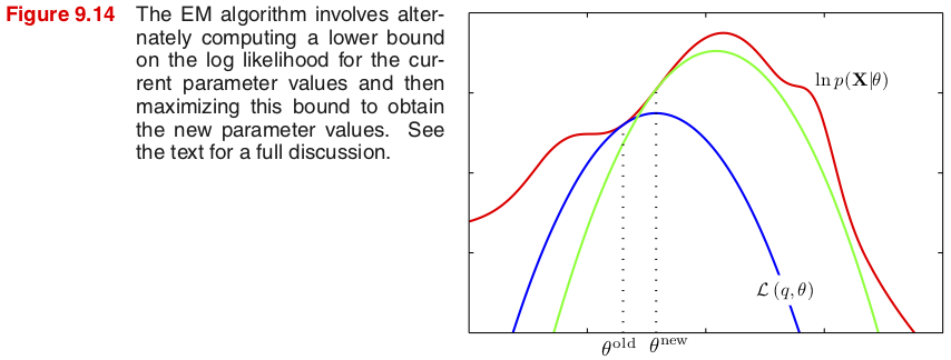
초기 모숫값 $\theta^{old}$에서 시작해보자. 먼저 (E step)에서 잠재변수에 대한 사후확률분포 $q(\bZ)=p(\bZ|\bX,\theta^{old})$를 구하게 된다. 그림에서 파란색 그래프는 이렇게 구한 $q$를 하계 $\L(q,\theta)$에 적용한 후 모수 $\theta$에 대한 함수로 표현한 것이다. 모숫값 $\btheta^{old}$에서 하계는 로그우도함수와 같아지고, 특히 이 점에서 하계와 로그우도함수의 그래프는 같은 접선을 가진다.
Note: 모숫값 $\theta^{old}$에서 $\KL(q\|p)$는 최소가 되므로 이 점에서 $\frac{\partial}{\partial\theta} \KL(q\|p)=0$이다. 따라서 $$ \frac{\partial}{\partial\theta}\Big|_{\theta=\theta^{old}} \ln p(\bX|\theta) = \frac{\partial}{\partial\theta}\Big|_{\theta=\theta^{old}} \bigl[ \L(q,\theta) + \KL(q\|p) \bigr] = \frac{\partial}{\partial\theta}\Big|_{\theta=\theta^{old}} \L(q,\theta) $$
(M step)에서 하계 $\L(q,\theta)$이 최대가 되는 모수 $\theta^{new}$를 찾는데, 이 점에서 파란색 그래프는 최대가 된다. 이어지는 (E step)에서 새로운 사후확률분포 $q'(\bZ)=p(\bZ|\bX,\theta^{new})$를 구하고 이를 적용한 하계 $\L(q',\theta)$ (녹색 그래프)는 $\theta^{new}$에서 다시 로그우도함수와 같은 접선을 가진다.