LaTeX new commands defined for this notebook: $ \newcommand{\bx}{\boldsymbol{x}} \newcommand{\N}{\mathcal{N}} \newcommand{\bmu}{\boldsymbol{\mu}} \newcommand{\bgamma}{\boldsymbol{\gamma}} \newcommand{\bSigma}{\boldsymbol{\Sigma}} \newcommand{\bz}{\boldsymbol{z}} \newcommand{\D}{\mathcal{D}} \newcommand{\bpi}{\boldsymbol{\pi}} \newcommand{\bI}{\boldsymbol{I}} \newcommand{\Mult}{\operatorname{Mult}} \newcommand{\bzero}{\boldsymbol{0}} $
\bx$\bx$,\N$\N$,\bmu$\bmu$,\bgamma$\bgamma$,\bSigma$\bSigma$,\bz$\bz$,\D$\D$,\bpi$\bpi$,\bI$\bI$,\Mult$\Mult$,\bzero$\bzero$
import numpy as np
import matplotlib as mpl
import matplotlib.pyplot as plt
%matplotlib inline

mpl.style.use('seaborn-white')
9.2 Mixtures of Gaussians
$K$개의 가우시안 확률밀도함수들이 선형 중첩된 형태를 가우시안 혼합모델(mixture of Gaussians)이라 부른다. $$ p(\bx) = \sum_k \pi_k \N(\bx|\bmu_k,\bSigma_k) \tag{9.7} $$
from mpl_toolkits.mplot3d import Axes3D

from scipy.stats import multivariate_normal, ortho_group

mu = np.asarray([[0.2, 0.4], [0.5, 0.5], [0.8, 0.6]])
lamb = np.asarray([0.02, 0.002])

ortho1 = np.asarray([[1, -1], [1,  1]]) / np.sqrt(2)
cov1 = ortho1 @ np.diag(lamb) @ ortho1.T

ortho2 = np.asarray([[1, 1], [-1,  1]]) / np.sqrt(2)
cov2 = ortho2 @ np.diag(lamb) @ ortho2.T

rv1 = multivariate_normal(mean=mu[0], cov=cov1)
rv2 = multivariate_normal(mean=mu[1], cov=cov2)
rv3 = multivariate_normal(mean=mu[2], cov=cov1)

def mixed_gaussian(x, pi=(0.5, 0.3, 0.2)):
    return pi[0] * rv1.pdf(x) + pi[1] * rv2.pdf(x) + pi[2] * rv3.pdf(x)

delta = 0.02
x, y = np.mgrid[0:1:delta, 0:1:delta]

fig = plt.figure(figsize=(13,4))

ax1 = fig.add_axes((0, 0, 0.25, 1))
ax1.set(aspect='equal', title='(a)')

cs1 = ax1.contour(x, y, rv1.pdf(np.dstack((x, y))), colors='C3', alpha=0.75)
ax1.clabel(cs1, inline=1, fontsize=8)

cs2 = ax1.contour(x, y, rv2.pdf(np.dstack((x, y))), colors='C2', alpha=0.75)
ax1.clabel(cs2, inline=1, fontsize=8)

cs3 = ax1.contour(x, y, rv3.pdf(np.dstack((x, y))), colors='C0', alpha=0.75)
ax1.clabel(cs3, inline=1, fontsize=8)

ax2 = fig.add_axes((0.3, 0, 0.25, 1))
ax2.set(aspect='equal', title='(b)')

cs4 = ax2.contour(x, y, mixed_gaussian(np.dstack((x, y))), colors='C4')
ax2.clabel(cs4, inline=1, fontsize=8)

ax3 = fig.add_axes((0.6, 0, 0.4, 1), projection='3d')
ax3.set_title('(c)')

x, y = np.mgrid[0:1:delta, 0:1:delta].reshape((2, -1))
ax3.plot_trisurf(x, y, mixed_gaussian(np.stack((x, y), axis=1)), cmap='coolwarm')
ax3.view_init(30, -60)

for ax in (ax1, ax2, ax3):
    ax.set(xlabel='$x_1$', ylabel='$x_2$', xlim=(0, 1), xticks=[0, 0.5, 1], yticks=[0, 0.5, 1])

Figure 2.23 Illustration of a mixture of 3 Gaussians in a two-dimensional space. (a) Contours of constant density for each of the mixture components, in which the 3 components are denoted red, green and blue, and the values of the mixing coefficients are 0.5, 0.3, 0.2, respectively. (b) Contours of the marginal probability density $p(\bx)$ of the mixture distribution. (c) A surface plot of the distribution $p(\bx)$.
Mixtures of Gaussians in terms of latent variables
이산 잠재변수 $\bz$를 도입해 가우시안 혼합모델을 설명해 보자.
(1-of-$K$ coding scheme) $K$개의 가우시안 확률밀도함수 $\N(\bx|\bmu_k,\bSigma_k)$ 중 어떤 것을 선택할 지는 ($K$-평균 알고리즘의 클러스터 라벨과 같이) 이진 확률변수 $\bz=(z_1,\dotsc,z_K)^T$를 이용한다. (단, $z_k\in\{0,1\}$이고 $\sum_k z_k=1$이 성립)
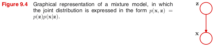
결합확률분포 $p(\bx,\bz)$는 주변확률분포 $p(\bz)$와 조건부분포 $p(\bx|\bz)$의 곱으로 나타나고, 그래프 모델은 그림 9.4와 같다.
주변확률분포 $p(\bz)$는 혼합계수(mixing coefficients) $\pi_k$를 이용해 다음과 같이 정의한다. $$ p(z_k=1) \equiv \pi_k \quad\Rightarrow\quad p(\bz) = \Mult(\bz|\bpi) \equiv \prod_k \pi_k^{z_k} \tag{9.10} $$ 이때 $p(\bz)$는 확률분포이므로 혼합계수는 $0\leq \pi_k\leq 1$과 $\sum_\bz p(\bz)=\sum_k \pi_k = 1$이 성립한다. ($\pi_k=0$일 때, $\pi_k^0\equiv 1$로 정의)
조건부분포 $p(\bx|\bz)$는 가우시안 분포로 정의한다. $$ p(\bx|z_k=1) \equiv \N(\bx|\bmu_k,\bSigma_k) \quad\Rightarrow\quad p(\bx|\bz) = \prod_k \N(\bx|\bmu_k,\bSigma_k)^{z_k} \tag{9.11} $$
가우시안 혼합모델은 (숨겨진) 잠재변수 $\bz$를 이용해 $\bx$의 주변확률분포로 표시할 수 있다. $$ p(\bx) = \sum_\bz p(\bx,\bz)= \sum_\bz p(\bz) p(\bx|\bz) = \sum_k \pi_k \N(\bx|\bmu_k,\bSigma_k) \tag{9.12} $$
조건부분포 $p(\bz|\bx)$는 $\bx$에 대한 성분 $\bz$의 신뢰도(responsibility)를 나타낸다. \begin{align*} p(\bz|\bx) &= \frac{p(\bz)p(\bx|\bz)}{p(\bx)} = \frac{\prod_k \bigl[\pi_k \N(\bx|\bmu_k,\bSigma_k)\bigr]^{z_k}}{\sum_j \pi_j \N(\bx|\bmu_j,\bSigma_j)} = \prod_k \left\{ \frac{\pi_k \N(\bx|\bmu_k,\bSigma_k)}{\sum_j \pi_j \N(\bx|\bmu_j,\bSigma_j)} \right\}^{z_k} \\ &\equiv \prod_k \gamma_k^{z_k} = \Mult(\bz|\bgamma) \tag{9.13} \end{align*} 즉, $\gamma_k \equiv \gamma(z_k) \equiv \dfrac{\pi_k \N(\bx|\bmu_k,\bSigma_k)}{\sum_j \pi_j \N(\bx|\bmu_j,\bSigma_j)}$는 $\bx$에 대한 $k$번째 성분의 신뢰도를 의미한다.
Ancestral sampling
For a directed acyclic graph (DAG) with $K$ nodes, the joint distribution over $K$ variables $\bx=\{x_1,\dotsc,x_K\}$ is given by $$ p(\bx) = \prod_k p(x_k|pa_k) \tag{8.5} $$ where $pa_k$ denotes the set of parents of $x_k$.
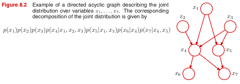
We shall suppose that the variables have been ordered such that there are no links from any node to any lower numbered node.
How to draw samples $\widehat{x}_1,\dotsc,\widehat{x}_K$ from the joint distribution $p(\bx)=p(x_1,\dotsc,x_K)$
- We start with the lowest-numbered node and draw a sample from the distribution $p(x_1)$, which we call $\widehat{x}_1$.
- We then work through each of the nodes in order, so that for node $n$ we draw a sample from the conditional distribution $p(x_n|pa_n)$ in which the parent variables $pa_n$ have been set to their sampled values.
- Once we have sampled from the final variable $x_K$, we will have achieved our objective of obtaining a sample from the joint distribution.
Generate random samples from a Gaussian mixture model with ancestral sampling
가우시안 혼합모델에서 무작위 샘플링은 앤세스터럴(ancestral) 샘플링 기법을 이용한다.
먼저 주변확률분포 $p(\bz)$로부터 잠재변수 $\bz$의 샘플 $\widehat{\bz}$를 추출한 후 조건부분포 $p(\bx|\widehat{\bz})$에서 $\bx$의 샘플을 추출한다.
결합확률분포 $p(\bx,\bz)$로부터 추출한 샘플(complete)은 그림 9.5(a)와 같이 $\bx$와 함께 $\bz$ 값을 색깔로 표시하면 된다.
주변확률분포 $p(\bx)$로부터 추출한 샘플(incomplete)은 그림 9.5(b)와 같이 결합확률분포 $p(\bx,\bz)$로부터 추출한 샘플에서 $\bz$ 값을 무시하고 (동일한 색으로) 표시하면 된다.
신뢰도 $\gamma(z_{nk})$는 그림 9.5(c)와 같이 샘플 $\bx_n$의 색깔을 나타낼 때 {R, G, B} 색상의 비율을 각각 {$\gamma(z_{n1})$, $\gamma(z_{n2})$, $\gamma(z_{n3})$}로 처리해서 표시하면 된다. 예를 들어, 신뢰도 $\gamma(z_{n1})=1$인 경우 색깔은 빨강(red)이 되고, $\gamma(z_{n2})=\gamma(z_{n3})=0.5$인 경우 시안(cyan)이 된다.
from scipy.stats import multinomial, multivariate_normal, ortho_group

mu = np.asarray([[0.2, 0.4], [0.5, 0.5], [0.8, 0.6]])
lamb = np.asarray([0.02, 0.002])

ortho1 = np.asarray([[1, -1], [1,  1]]) / np.sqrt(2)
cov1 = ortho1 @ np.diag(lamb) @ ortho1.T

ortho2 = np.asarray([[1, 1], [-1,  1]]) / np.sqrt(2)
cov2 = ortho2 @ np.diag(lamb) @ ortho2.T

rvs = (multivariate_normal(mean=mu[0], cov=cov1),
       multivariate_normal(mean=mu[1], cov=cov2),
       multivariate_normal(mean=mu[2], cov=cov1))

K = 3
pi = (0.5, 0.3, 0.2)

resp = lambda x: \
    [pi[k] * rvs[k].pdf(x) / np.sum([pi[j] * rvs[j].pdf(x) for j in range(K)]) for k in range(K)]

fig, ax = plt.subplots(ncols=3, figsize=(13,4))

N = 500
z = np.nonzero(multinomial.rvs(1, pi, size=N))[1] # do not use one-hot encoding
x = np.array([rvs[z[i]].rvs() for i in range(N)])

for k in range(K):
    xz = x[np.argwhere(z == k).squeeze()]
    ax[0].plot(*xz.T, 'o', markersize=4, color=np.identity(3)[k])

ax[1].plot(*x.T, 'o', markersize=4, color=(1,0,1)) # magenta

ax[2].scatter(*x.T, s=16, c=[resp(n) for n in x])

for i, iax in enumerate(ax):
    iax.set(aspect='equal', xlim=(0, 1), ylim=(0, 1), xticks=[0, 0.5, 1], yticks=[0, 0.5, 1],
            title='({})'.format(chr(ord('a')+i)))

Figure 9.5 Example of 500 points drawn from the mixture of 3 Gaussians shown in Figure 2.23. (a) Samples from the joint distribution $p(\bz)p(\bx|\bz)$ in which the three states of $\bz$, corresponding to the three components of the mixture, are depicted in red, green, and blue, and (b) the corresponding samples from the marginal distribution $p(\bx)$, which is obtained by simply ignoring the values of $\bz$ and just plotting the $\bx$ values. The data set in (a) is said to be complete, whereas that in (b) is incomplete. (c) The same samples in which the colours represent the value of the responsibilities $\gamma(z_{nk})$ associated with data point $\bx_n$, obtained by plotting the corresponding point using proportions of red, green, and blue ink given by $\gamma(z_{nk})$ for $k=1,2,3$, respectively.
9.2.1 Maximum likelihood
주어진 관측 데이터 $\D=\{\bx_1,\dotsc,\bx_N\}$를 가장 잘 표현해 주는 가우시안 혼합모델을 찾는 것이 목적이다.
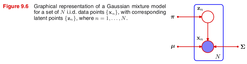
이때 가우시안 혼합모델을 결정하는 모수는 혼합계수 $\bpi$, 평균 $\bmu$, 공분산 $\bSigma$이고, 관측 데이터들이 i.i.d.라고 가정하면 그래프 모델은 그림 9.6과 같다.
가우시안 혼합모델의 로그우도함수를 최대가 되게 하는 모수를 최대우도추정으로 구해 보자. $$ \ln p(\D|\bpi,\bmu,\bSigma) = \sum_n \ln \left\{ \sum_k \pi_k \N(\bx_n|\bmu_k,\bSigma_k) \right\} \tag{9.14} $$
MLE for mean $\bmu_k$
$$ \bmu_k^{ML} = \frac{1}{N_k} \sum_n \gamma(z_{nk}) \bx_n \quad\text{where}\quad N_k = \sum_n \gamma(z_{nk}) \tag{9.17-18} $$
Note: (1) $N_k$는 각 데이터에 대한 성분 $k$의 신뢰도를 모두 합한 값이다. (2) $\bmu_k^{ML}$은 데이터들의 가중평균으로 가중치는 사후확률 $\gamma(z_{nk})=p(z_k=1|\bx_n)$, 또는 데이터 $\bx_n$에 대한 성분 $k$의 신뢰도로 주어졌다.
Proof. 행렬 미분(Appendix C)을 이용해 가우시안 분포를 $\bmu_k$에 대해 편미분하면 \begin{align*} \frac{\partial}{\partial\bmu_k} \N(\bx_n|\bmu_k,\bSigma_k) &= \N(\bx_n|\bmu_k,\bSigma_k) \cdot \frac{\partial}{\partial\bmu_k} \left\{ -\frac{1}{2}(\bx_n-\bmu_k)^T\bSigma_k^{-1}(\bx_n-\bmu_k) \right\} \\ &= \N(\bx_n|\bmu_k,\bSigma_k)\cdot \bSigma_k^{-1}(\bx_n-\bmu_k) \end{align*} 이고, 로그우도함수의 미분이 $\bzero$이 되는 모수 $\bmu_k$를 구해보면 \begin{align*} \bzero = \dfrac{\partial}{\partial\bmu_k} \ln p(\D|\bpi,\bmu,\bSigma) &= \sum_n \frac{\bpi_k\frac{\partial}{\partial\bmu_k}\N(\bx_n|\bmu_k,\bSigma_k)}{ \sum_j \pi_j \N(\bx_n|\bmu_j,\bSigma_j) } \\ &= \sum_n \frac{\bpi_k\N(\bx_n|\bmu_k,\bSigma_k)}{ \sum_j \pi_j \N(\bx_n|\bmu_j,\bSigma_j) } \cdot \bSigma_k^{-1}(\bx_n-\bmu_k) \\ &= \sum_n \gamma(z_{nk}) \cdot \bSigma_k^{-1}(\bx_n-\bmu_k) \tag{9.16} \end{align*} 양 변에 $\bSigma_k$를 곱하면 $\bzero = \sum_n \gamma(z_{nk}) (\bx_n-\bmu_k)$. 따라서 $\bigl[\sum_n \gamma(z_{nk})\bigr] \bmu_k = N_k \bmu_k = \sum_n \gamma(z_{nk})\bx_n$이다.
MLE for covariance $\bSigma_k$
$$ \bSigma_k^{ML} = \frac{1}{N_k} \sum_n \gamma(z_{nk}) (\bx_n-\bmu_k)(\bx_n-\bmu_k)^T \tag{9.19} $$
MLE for mixing coefficient $\pi_k$
$$ \pi_k^{ML} = \frac{N_k}{N} \tag{9.22} $$
9.2.2 EM for Gaussian mixtures
최대우도추정으로 구한 세 가지 모수 $\bmu_k^{ML}$, $\bSigma_k^{ML}$, $\pi_k^{ML}$을 계산하려면 먼저 신뢰도 $\gamma(z_{nk})$를 구하여야 한다. 하지만 (9.13)에서 정의된 신뢰도는 세 가지 모수들이 서로 얽혀 있는 복잡한 형태로 나타나므로 (닫힌 형태의 식으로 표현되지 않으므로) 간단히 계산할 수 없다.
따라서 (E step) 현재의 모수 값으로 (9.13)을 이용해 사후확률인 신뢰도 $\gamma(z_{nk})$를 구하고, (M step) 새롭게 구한 신뢰도를 이용해 (9.17), (9.19), (9.22)를 이용해 세 가지 모수 $\bmu_k$, $\bSigma_k$, $\pi_k$의 최대우도추정을 하려고 한다.
EM for Gaussian Mixtures
Given a Gaussian mixture model, the goal is to maximize the likelihood function with respect to the parameters (comprising the means and covariances of the components and the mixing coefficients).
- Initialize the means $\bmu_k$, covariances $\bSigma_k$ and mixing coefficients $\pi_k$, and evaluate the initial value of the log likelihood.
- (E step) Evaluate the responsibilities using the current parameter values $$ \gamma(z_{nk}) = \frac{\pi_k \N(\bx|\bmu_k,\bSigma_k)}{\sum_j \pi_j \N(\bx|\bmu_j,\bSigma_j)} \tag{9.23} $$
- (M step) Re-estimate the parameters using the current responsibilities \begin{align*} \bmu_k^{new} &= \frac{1}{N_k} \sum_n \gamma(z_{nk}) \bx_n \tag{9.24} \\ \bSigma_k^{new} &= \frac{1}{N_k} \sum_n \gamma(z_{nk}) (\bx_n-\bmu_k^{new})(\bx_n-\bmu_k^{new})^T \tag{9.25} \\ \pi_k^{new} &= \frac{N_k}{N} \tag{9.26} \end{align*} where $$ N_k = \sum_n \gamma(z_{nk}) \tag{9.27} $$
- Evaluate the log likelihood $$ \ln p(\D|\bpi,\bmu,\bSigma) = \sum_n \ln \left\{ \sum_k \pi_k \N(\bx_n|\bmu_k,\bSigma_k) \right\} \tag{9.28} $$ and check for convergence of either the parameters or the log likelihood. If the convergence criterion is not satisfied return to Step 2.
from pandas import read_csv
from sklearn.preprocessing import scale

data = read_csv('data/Old_Faithful.csv', header=None).values
data_scaled = scale(data)

from scipy.stats import multivariate_normal
from matplotlib.patches import Circle
from matplotlib.collections import PatchCollection

K = 2

pi_init = np.array((0.5, 0.5))
mu_init = np.array([[-1.5, 1], [1.5, -1]])
var_init = 0.5 * np.identity(2)
cov_init = np.array((var_init, var_init))

def draw_multivariate_normal(ax, mu, cov):
    delta = 0.05
    x, y = np.mgrid[-2.5:2.5:delta, -2.5:2.5:delta]
    z0 = multivariate_normal.pdf(np.dstack((x, y)), mean=mu[0], cov=cov[0])
    z1 = multivariate_normal.pdf(np.dstack((x, y)), mean=mu[1], cov=cov[1])
    level0 = np.exp(-0.5) / (2. * np.pi) / np.sqrt(np.linalg.det(cov[0]))
    level1 = np.exp(-0.5) / (2. * np.pi) / np.sqrt(np.linalg.det(cov[1]))
    ax.contour(x, y, z0, levels=[level0], linewidths=6, colors=[(1,1,1)])
    ax.contour(x, y, z0, levels=[level0], linewidths=2, colors=[(0,0,1)])
    ax.contour(x, y, z1, levels=[level1], linewidths=6, colors=[(1,1,1)])
    ax.contour(x, y, z1, levels=[level1], linewidths=2, colors=[(1,0,0)])

def mixed_colors(resp):
    return np.c_[resp[:,1], np.zeros(resp.shape[0]), resp[:,0]]

def E_step(x, pi, mu, cov):
    z = np.array([pi[k] * multivariate_normal.pdf(x, mean=mu[k], cov=cov[k]) for k in range(K)])
    return (z / np.sum(z, axis=0)).T

def M_step(x, resp):
    N = x.shape[0]
    N_k = np.sum(resp, axis=0)
    mu = np.array([ np.sum(resp[:,(k,)] * x, axis=0) / N_k[k] for k in range(K) ])
    cov = np.array([ np.sum([resp[i, k] * np.outer(x[i] - mu[k], x[i] - mu[k]) for i in range(N)], axis=0) / N_k[k]
        for k in range(K) ])
    pi = N_k / N
    return pi, mu, cov

fig, ax = plt.subplots(nrows=2, ncols=3, figsize=(12,8.5), sharex=True, sharey=True,
                       gridspec_kw=dict(wspace=0.05, hspace=0.1))
ax = ax.ravel()

pi = pi_init
mu = mu_init
cov = cov_init

ax[0].plot(*data_scaled.T, 'o', markersize=4, color=(0,1,0))
draw_multivariate_normal(ax[0], mu, cov)

resp = E_step(data_scaled, pi, mu, cov)
ax[1].scatter(*data_scaled.T, s=16, c=mixed_colors(resp))
draw_multivariate_normal(ax[1], mu, cov)

L = 1
pi, mu, cov = M_step(data_scaled, resp)
ax[2].scatter(*data_scaled.T, s=16, c=mixed_colors(resp), label='$L={}$'.format(L))
draw_multivariate_normal(ax[2], mu, cov)

L = 2
resp = E_step(data_scaled, pi, mu, cov)
pi, mu, cov = M_step(data_scaled, resp)
ax[3].scatter(*data_scaled.T, s=16, c=mixed_colors(resp), label='$L={}$'.format(L))
draw_multivariate_normal(ax[3], mu, cov)

for _ in range(3):
    L += 1
    resp = E_step(data_scaled, pi, mu, cov)
    pi, mu, cov = M_step(data_scaled, resp)
ax[4].scatter(*data_scaled.T, s=16, c=mixed_colors(resp), label='$L={}$'.format(L))
draw_multivariate_normal(ax[4], mu, cov)

for _ in range(15):
    L += 1
    resp = E_step(data_scaled, pi, mu, cov)
    pi, mu, cov = M_step(data_scaled, resp)
ax[5].scatter(*data_scaled.T, s=16, c=mixed_colors(resp), label='$L={}$'.format(L))
draw_multivariate_normal(ax[5], mu, cov)

for i, iax in enumerate(ax):
    iax.set(aspect='equal', xlim=(-2.5, 2.5), ylim=(-2.5, 2.5), xticks=(-2, 0, 2), yticks=(-2, 0, 2),
            title='({})'.format(chr(ord('a')+i)))
    if i >= 2:
        iax.legend()

Figure 9.8 Illustration of the EM algorithm using the Old Faithful set as used for the illustration of the $K$-means algorithm in Figure 9.1.
- Plot (a) shows the data points in green, together with the initial configuration of the mixture model in which the one standard-deviation contours ($c=\frac{\exp(-1/2)}{2\pi|\Sigma|^{1/2}}$) for the two Gaussian components are shown as blue and red circles.
NOTE: $\N(\bx|\bmu_k,\bSigma_k)$ has density $\frac{1}{\sqrt{(2\pi)^D|\bSigma_k|}}\exp\bigl\{-\frac{1}{2}(\bx-\bmu_k)^T\bSigma_k^{-1}(\bx-\bmu_k)\bigr\}$. Here the one standard-deviation contours means the set of points $\bx$ such that the Mahalanobis distance $\sqrt{(\bx-\bmu_k)^T\bSigma_k^{-1}(\bx-\bmu_k)}=1$. In case when $D=1$, the Mahalanobis distance reduces to the absolute value of the standard score $\frac{|x-\mu_k|}{\sigma}=1$.
- Plot (b) shows the result of the initial E step, in which each data point is depicted using a proportion of blue ink equal to the posterior probability of having been generated from the blue component, and a corresponding proportion of red ink given by the posterior probability of having been generated by the red component. Thus, points that have a significant probability for belonging to either cluster appear purple.
- The situation after the first M step is shown in plot (c), in which the mean of the blue Gaussian has moved to the mean of the data set, weighted by the probabilities of each data point belonging to the blue cluster, in other words it has moved to the centre of mass of the blue ink. Similarly, the covariance of the blue Gaussian is set equal to the covariance of the blue ink. Analogous results hold for the red component.
- Plots (d), (e), and (f) show the results after 2, 5, and 20 complete cycles of EM, respectively. In plot (f) the algorithm is close to convergence.
$K$-means algorithm for initialization
EM 알고리즘은 $K$-평균 알고리즘에 비해 수렴하는데 더 많은 반복 횟수가 필요할뿐 아니라 반복 사이클마다 더 많은 계산이 요구된다. 그러므로 가우시안 혼합모델을 위한 모수들의 초기값을 $K$-평균 알고리즘으로 찾은 후 EM 알고리즘을 실행하는 것이 일반적이다.
평균 $\bmu_k$의 초기값은 $K$-평균 알고리즘이 찾은 클러스터 센터로 지정하면 된다. $K$-평균 알고리즘은 관측 데이터들을 $K$개의 클러스터로 분류하므로 각 클러스터들의 샘플 공분산을 $\bSigma_k$의 초기값으로 줄 수 있다. 또한 혼합계수 $\pi_k$의 초기값은 각 클러스터에 속한 데이터의 수를 전체 데이터의 수로 나눈 값으로 지정하면 된다.
로그우도함수는 여러 개의 극댓값을 가질 수 있으므로 EM 알고리즘으로 찾은 수렴값이 항상 최대라는 보장은 할 수 없다.
from sklearn.cluster import k_means
from scipy.stats import multivariate_normal

K = 2
N = data_scaled.shape[0]

mu_init, labels, _ = k_means(data_scaled, K)
cov_init = np.array([np.cov(data_scaled[labels == k].T) for k in range(K)])
pi_init = np.array([data_scaled[labels == k].shape[0] for k in range(K)]) / N

def draw_multivariate_normal(ax, mu, cov):
    delta = 0.05
    x, y = np.mgrid[-2.5:2.5:delta, -2.5:2.5:delta]
    z0 = multivariate_normal.pdf(np.dstack((x, y)), mean=mu[0], cov=cov[0])
    z1 = multivariate_normal.pdf(np.dstack((x, y)), mean=mu[1], cov=cov[1])
    level0 = np.exp(-0.5) / (2. * np.pi) / np.sqrt(np.linalg.det(cov[0]))
    level1 = np.exp(-0.5) / (2. * np.pi) / np.sqrt(np.linalg.det(cov[1]))
    ax.contour(x, y, z0, levels=[level0], linewidths=6, colors=[(1,1,1)])
    ax.contour(x, y, z0, levels=[level0], linewidths=2, colors=[(0,0,1)])
    ax.contour(x, y, z1, levels=[level1], linewidths=6, colors=[(1,1,1)])
    ax.contour(x, y, z1, levels=[level1], linewidths=2, colors=[(1,0,0)])

def mixed_colors(resp):
    return np.c_[resp[:,1], np.zeros(resp.shape[0]), resp[:,0]]

def E_step(x, pi, mu, cov):
    z = np.array([pi[k] * multivariate_normal.pdf(x, mean=mu[k], cov=cov[k]) for k in range(K)])
    return (z / np.sum(z, axis=0)).T

def M_step(x, resp):
    N = x.shape[0]
    N_k = np.sum(resp, axis=0)
    mu = np.array([ np.sum(resp[:,(k,)] * x, axis=0) / N_k[k] for k in range(K) ])
    cov = np.array([ np.sum([resp[i, k] * np.outer(x[i] - mu[k], x[i] - mu[k]) for i in range(N)], axis=0) / N_k[k]
        for k in range(K) ])
    pi = N_k / N
    return pi, mu, cov

def log_likelihood(x, pi, mu, cov):
    return np.sum(np.log(np.sum(
        [pi[k] * multivariate_normal.pdf(x, mean=mu[k], cov=cov[k]) for k in range(K)], axis=0)))

fig = plt.figure(figsize=(10,3.5))

pi = pi_init
mu = mu_init
cov = cov_init

L = 0
resp = E_step(data_scaled, pi, mu, cov)

ax1 = fig.add_axes((0, 0, 0.3, 1))
ax1.scatter(*data_scaled.T, s=16, c=mixed_colors(resp), label='$L={}$'.format(L))
draw_multivariate_normal(ax1, mu, cov)
ax1.set_title('Initialize with K-means')

pdf = [log_likelihood(data_scaled, pi, mu, cov)]
for _ in range(5):
    L += 1
    resp = E_step(data_scaled, pi, mu, cov)
    pi, mu, cov = M_step(data_scaled, resp)
    pdf.append(log_likelihood(data_scaled, pi, mu, cov))

ax2 = fig.add_axes((0.34, 0, 0.3, 1))
ax2.scatter(*data_scaled.T, s=16, c=mixed_colors(resp), label='$L={}$'.format(L))
draw_multivariate_normal(ax2, mu, cov)
ax2.set_title('After {} cycles of EM'.format(L))

ax3 = fig.add_axes((0.72, 0.1, 0.28, 0.8))
ax3.plot(pdf, 'o-')
ax3.set(xlabel='$L$', yticks=np.arange(-387, -384), title='log likelihood')

for ax in (ax1, ax2):
    ax.set(aspect='equal', xlim=(-2.5, 2.5), ylim=(-2.5, 2.5), xticks=(-2, 0, 2), yticks=(-2, 0, 2))
    ax.legend()

Singularity problem in a Gaussian mixture
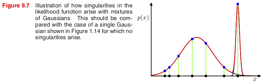
가우시안 혼합모델($K\geq 2$)의 최대우도추정에는 특이점이 발생해 그 점으로 확률밀도가 쏠릴 수 있는 심각한 문제가 있다.
손쉬운 계산을 위해 공분산 행렬은 $\bSigma_k = \sigma_k^2\bI$로 두자. 만약 관측 데이터 중 하나가 정확히 평균들 중 하나와 일치한다면 ($\bx_n=\bmu_k$), 이 점에서 확률밀도는 $$ p(\bx_n) = \N(\bx_n|\bx_n,\sigma_k^2\bI) = \frac{1}{(2\pi)^{D/2}}\frac{1}{\sigma_k^D} \tag{9.15} $$ 따라서 로그우도 $\ln p(\bx_n)\to\infty$ as $\sigma_k\to0$.
그렇다면 $\sigma_k$를 줄이면 줄일수록 로그우도가 계속 증가하는데, 이것이 최대우도를 추정하는데 영향을 미치지 않을까?
하나의 가우시안 분포로만 이루어진 모델($K=1$)에서는 문제가 없다.
NOTE: 다른 데이터 $\bx\neq\bmu_k$의 경우 $$ \ln p(\bx) = C_0 - D\ln\sigma_k - C(\bx)\sigma_k^{-2} \to -\infty \quad\text{as}\quad \sigma_k\to0 $$ where $C_0 = -\frac{D\ln(2\pi)}{2}$ and $C(\bx) = \frac{\|\bx-\bmu_k\|^2}{2}$. 따라서 $\bx\neq\bmu_k$인 데이터가 하나만 있어도 로그우도의 합은 음의 무한대로 접근하므로 최대우도를 추정하는데 아무런 영향을 미치지 않는다.
이제 $K=2$일 때 $\sigma_1$을 유한한 값으로 고정하고 $\sigma_2$를 0에 가깝게 줄여보자. 만약 특정한 데이터 $\bx_n$이 두 번째 평균 $\bmu_2$와 같다면 (즉, 특이점이 발생한다면) \begin{align*} \ln p(\bx_n) &= \ln \bigl( \pi_1 \N(\bx_n|\bmu_1,\sigma_1^2\bI) + \pi_2 \N(\bx_n|\bmu_2,\sigma_2^2\bI) \bigr) \\ &= \ln \left\{ \frac{\pi_1}{(2\pi)^{D/2}}\cdot\frac{1}{\sigma_1^D}\exp\Bigl(\frac{-\|\bx_n-\bmu_1\|^2}{2\sigma_1^2}\Bigr) + \frac{\pi_2e^{-1/2}}{(2\pi)^{D/2}}\cdot\frac{1}{\sigma_2^D} \right\} \to \infty \quad\text{as}\quad \sigma_2\to 0 \end{align*} 그런데 $\bx\neq\bmu_2$인 데이터들의 경우 $\frac{1}{\sigma_2^D}\exp\Bigl(\frac{-\|\bx-\bmu_2\|^2}{2\sigma_2^2}\Bigr)\to 0$ as $\sigma_2\to0$ 이므로 \begin{align*} \ln p(\bx) &= \ln \left\{ \frac{\pi_1}{(2\pi)^{D/2}}\cdot\frac{1}{\sigma_1^D}\exp\Bigl(\frac{-\|\bx-\bmu_1\|^2}{2\sigma_1^2}\Bigr) + \frac{\pi_2}{(2\pi)^{D/2}}\cdot\frac{1}{\sigma_2^D}\exp\Bigl(\frac{-\|\bx-\bmu_2\|^2}{2\sigma_2^2}\Bigr) \right\} \\ &\to \ln \left\{ \frac{\pi_1}{(2\pi)^{D/2}}\cdot\frac{1}{\sigma_1^D}\exp\Bigl(\frac{-\|\bx-\bmu_1\|^2}{2\sigma_1^2}\Bigr) \right\} < \infty \quad\text{as}\quad \sigma_2\to 0 \end{align*} 따라서 $\sum_n \ln p(\bx_n) \to \infty$ as $\sigma_2\to 0$. 즉, 그림 9.7에서와 같이 특이점이 발생할 경우 $\sigma_2$를 줄이면 줄일수록 가우시안 혼합모델의 로그우도는 무한대로 증가한다.
결국 $K\geq2$인 가우시안 혼합모델에서는 최대우도추정 과정에서 특이점이 발생하는 (관측 데이터 중 하나가 정확히 평균들 중 하나와 일치하는) 경우 심각한 문제가 야기될 수 있다. 이와 같은 특이점 문제는 최대우도추정에서 나타날 수 있는 오버피팅의 단적인 예들 중 하나로 볼 수 있다. 하지만 베이지안 방법을 사용하는 경우에는 특이점 문제가 발생하지 않는다.
따라서 가우시안 혼합모델에서 최대우도추정을 할 때에는 특이점이 발생하지 않도록 휴리스틱한 방법을 고려해야 한다. 예를 들어, 가우시안 혼합모델의 특정한 컴포넌트에서 특이점이 발생하는 지 체크하고, 문제가 발생할 경우 이 컴포넌트의 평균을 무작위로 다시 고르고 공분산도 큰 값으로 재설정한 후 다시 최대우도추정을 하는 방법이다.
Identifiability problem in a Gaussian mixture
가우시안 혼합모델에서 최대우도추정을 하는데 나타나는 또 다른 문제점은, 동일한 최대우도추정 해답이 $K!$번 나타날 수 있다는 것이다. 예를 들어, $K=2$일 경우 최대우도추정으로 찾은 모수들의 컴포넌트 인덱스($k$)를 서로 바꾸면, 즉 $\pi_1\leftrightarrow\pi_2$, $\bmu_1\leftrightarrow\bmu_2$, $\bSigma_1\leftrightarrow\bSigma_2$, 최대우도를 주는 새로운 모수를 하나 더 얻을 수 있다. 이러한 경우 최대우도추정으로 찾은 모수들을 해석하는데 어려움이 발생할 수 있다.
-
A model that fails to be identifiable is said to be non-identifiable or unidentifiable: two or more parametrizations are observationally equivalent.